Papers I've read this week

This is a grab bag of papers. No theme, just what I found interesting. I’ve had a bunch of tabs open and finally (finally) got through them.

I hope to write more frequently going forward: the goal is once per month. My darling toddler has not been sleeping consistently, so my writing time has been exceptionally limited. Currently this has improved, and with luck, will stay improved.

Training LLMs over Neurally Compressed Text

[abstract]

The authors train LLMs over compressed text. When training language models, the current paradigm doesn’t involve raw text, but instead, trains the model over sequences of tokens, which are, basically, compressed text. The most common tokenizer is BPE (used by GPT-3, Llama/Mistral, etc.). The idea behind tokenization is that tokenizers transform the raw text into a much more efficient representation: BPE is typically 4x more efficient than raw bytes, so the LLM sees 4x the data for a given computational budget.

The natural question, then, is: why stop at 4x? Is there something better than BPE? There really hasn’t been— almost every LLM uses BPE for tokenization, although, as usual, there’s a lack of details about the latest foundation models. In the limit, a perfect compression algorithm should remove all predictable information from the sequence of bytes, so that shouldn’t be predictable, but could a tokenizer that’s, say, 8x more efficient than raw text be 2x as good as BPE?

The authors use a variety of compression techniques to train LLMs on ever more compressed text, looking at:

• GZip

• LLM based compression (which achieved a 12x compression ratio!).

• Arithmetic encoding with logits conditioned on the sequence of text seen so far, i.e.

  \(\hat{p}(x_i | x_0, \ldots, x_{i-1})\)

• Arithmetic encoding with static logits, i.e.

  \(\hat{p}(x_i | x_0, \ldots, x_{i-1}) = \hat{p}(x_i)\)

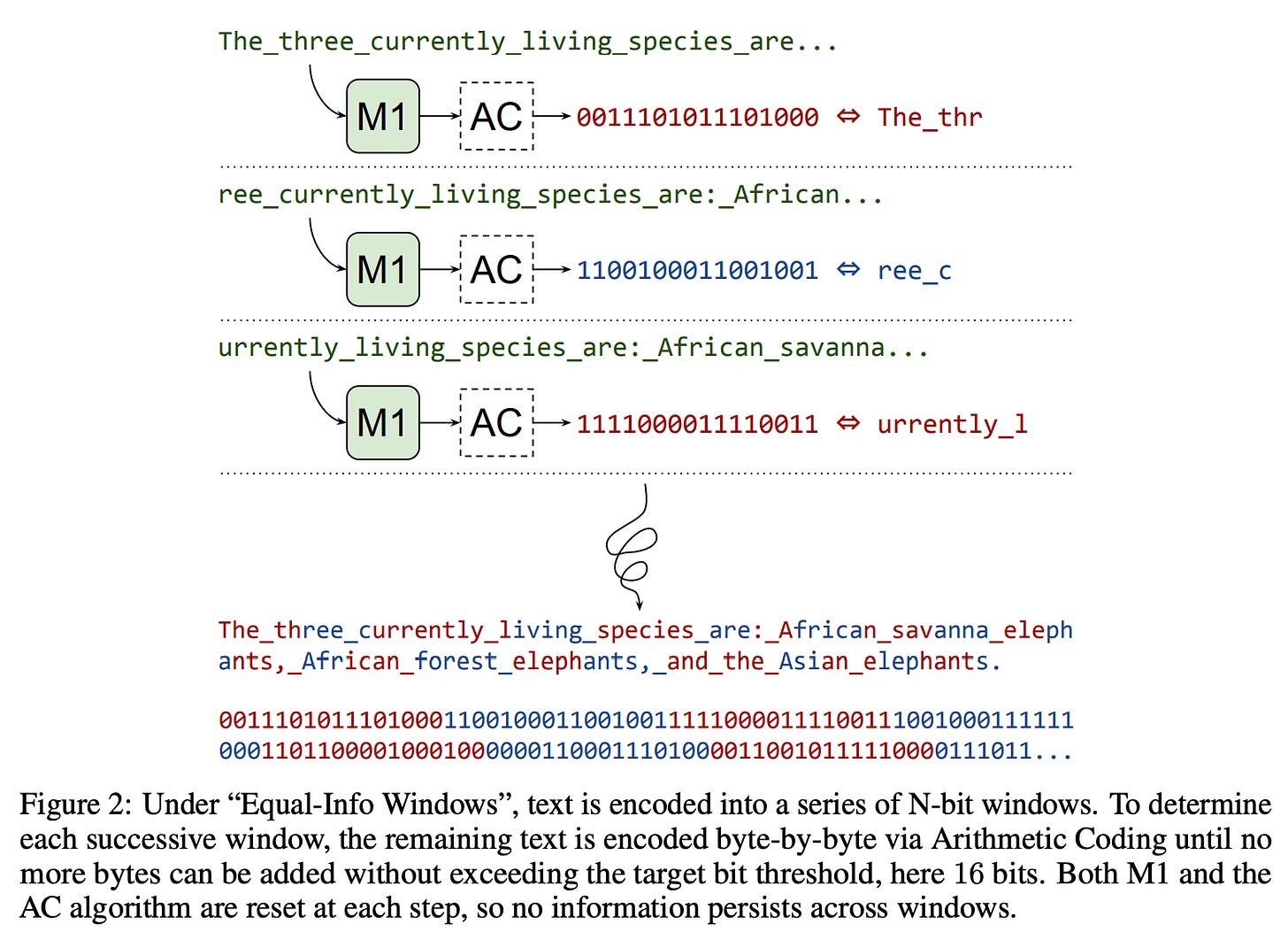
They also use a technique which they developed, that splits the text into equal sized windows that each contain 32 bits of compressed information.

They find that their best models underperform subword baselines, and all the compression schemes (including GZip, which I found surprising) are learnable by standard LLMs, but the performance is worse than standard sub-word tokenizers, like BPE. However, their method does outperform byte-level baselines.

To a certain extent, this is unsurprising; the goal behind compression is to remove any predictable patterns from the original sequence of bytes, so if we had a perfect compressor, the resulting output would be indistinguishable from random noise. What is surprising, though, is that BPE just happens to be the sweet spot for compression.

How arithmetic coding works is:

1. A message is represented by an interval of real numbers between 0 and 1.

2. As the message grows, the interval needed to represent it becomes smaller, so the number of bits needed grows.

3. you take as inputs an alphabet, which assigns a cardinality to the characters (i.e. an ordering from 0 to n) and a model that assigns probabilities to the characters from the alphabet conditioned on the previous characters in the sequence, i.e.

   \(p(x_t | x_1, \ldots, x_{t-1})\)

4. Finally, we get an interval of two floating point numbers that represent the number.

The original paper has a great example describing exactly how this works. The key takeaway is that arithmetic coding presents a way to use a probability distribution to compress text, and the better that our model represents the underlying distribution over characters, the more efficient the message.

The authors train a 3M parameter decoder in a fairly standard way, and use encoder

They use equal information windows, where they encode text into a series of N-bit windows, resetting the AC encoder when it can no longer add bits without exceeding the target bit threshold. Windows represent variable amounts of text, but should represent the same amount of information.

Once they have the compressed sequence of bits, they then create tokens by grouping every N bits into a token, creating a vocabulary of size 2^N. They try with N = 8 and N = 16. This seems suboptimal to me— there’s no semantic meaning to the tokens!

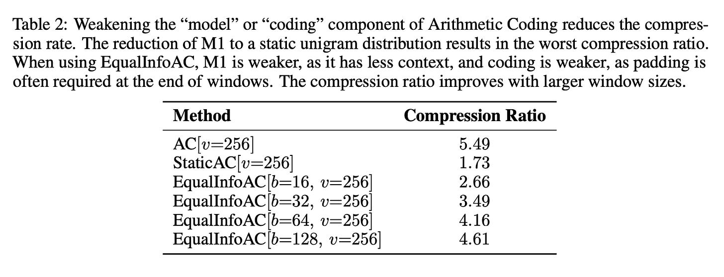
The paper has a fascinating table showing how each of these changes weakens the compression ratios:

The authors make a point of using the same hyperparameters for every training run they do. I think this is a mistake; a proper benchmark would tune the hyperparameters for each setting.

Their results are interesting:

• ArithmeticCoding and StaticAC settings are “essentially unlearnable”, failing to outperform their naive baseline which assigns equal probability to all tokens (aside: I love this baseline. more papers should include dumb heuristic baselines. we had a “UniformRandom” baseline agent in all our game theory papers and it performed remarkably well.)

• EqualInfoAC performs the best, coming close to matching SentencePiece.

They have some really interesting ablations, which show that the SentencePiece tokens are much more semantically relevant than EqualInfoAC:

The other ablations are fascinating. This was an excellent paper with strong empirical work. I would encourage you to read it.

Mixture of Depths

[abstract]

A windmill that is constantly being tilted at in decoder-centric LLM research is the fact that each token receives the same amount of compute. This seems clearly wrong. This paper proposed a novel method, Mixture of Depths (MoD), that dynamically allocates FLOPs to specific positions in a sequence.

The obvious comparison is to the Mixture of Experts (MoE) models. The MoD method can be thought of as using the routing logic from MoE models, but deploying a single expert with dynamic skipping based on the routing logic.

At a high level, the algorithm is:

1. Determine a compute budget which limits the number of tokens in a sequence that participate in a given block (say: 50% of the sequence participates in self-attention).

2. Use a per-block router to emit scalar weights for each token.

3. Select the top-k weights per block and sequence to participate in the block’s computation.

Note how similar this is to a MoE model.

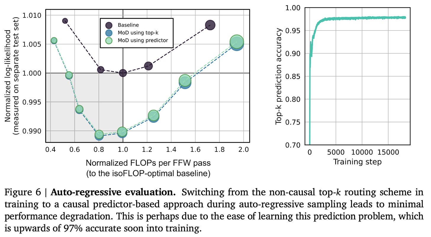
They use expert choice routing, as it removes the need for the oft-complicated auxiliary losses which are required for token-choice routing. The big problem, of course, is that the top-k operation is non-causal, which is why expert-choice routing isn’t used in any (published) MoE papers. They use a causal predictor-based approach, which has minimal degradation:

Their results are nice; they find that MoD is a nice improvement, lowering loss compared to the isoFLOP vanilla model. Additionally, they find that the MoD improvements compound with the improvements from training a MoE model:

The implications of this paper are fascinating; one can imagine a family of ever more complex routing mechanisms which let every decision become learned.

Sparse Upcycling: Training MoE models from dense checkpoints

[abstract]

The paper proposes a method to initialize a MoE model from a dense one, showing that this outperforms the original, dense model with only using 50% of the original compute, and also outperforming MoE models trained from scratch with the same compute budget.

The paper makes the fascinating observation that the vast majority of SOTA neural network are trained from scratch, which, in many ways, is assumed to be the default way that all models are trained. Given the lottery ticket hypothesis, it’s not at all clear that this is optimal. Even though the weights are chosen randomly, this doesn’t mean that they’re good; the joke that RL researchers like to make that the random seed is a crucial hyperparameter is actually a valid tactic to take when deploying systems into production. If OpenAI could produce a better ChatGPT by using seed 3 rather than seed 5, they’d absolutely do that.

In any case, the paper explores developing cheaper ways of training large models by using existing models. This is much more relevant now than when the paper was released (ICLR 2023, so the work was probably done in the second half of 2022): we’re training much larger models with much more compute and doing so much more often.

Generally speaking, Mixture of Experts work by having N copies of each layer (we call each copy an expert), and learning to allocate tokens to each expert. The upcycling algorithm that they propose creates a MoE model by expanding a subset of the MLP layers in the original, dense model into MoE layers, and copying the remaining layers of the dense model across to the MoE. Each expert is then initialized identically, as a copy of the original MLP, and the routers are randomly initialized. They continue training the model using the same hyperparameters (batch size, learning rate, etc.). They even find that resuming the optimizer state from the original dense checkpoint works well, which I find surprising.

The results are, bluntly, quite good. The slope of improvement in the validation metrics seems to change immediately. It seems as if by upcycling the model, new avenues of performance are immediately unlocked.

Given the earlier results from the Mixture of Depths paper, which suggested that MoD models compose with MoE models, this suggests a natural experiment: train a MoD model to some level of performance, and then upcycle it to a MoE/MoD model. As an engineer, I shudder at the resulting complexity, but it should have a significant jump in performance.

Replication of Chinchilla

https://twitter.com/borgeaud_s/status/1780988694163321250

[abstract]

Finally, this was quite short, but an exciting development that gave me faith in research. A team at Epoch AI, an independent research institute that does excellent work, tried reproducing Chinchilla by transcribing the data from the pixels of the chart. Let me repeat that: they reproduced Chinchilla by transcribing the data from the pixels of the original paper. And! What’s more! They found an error in the paper that caused the original authors to issue a correction and promise to release the data. Truly excellent work on their behalf.

The root of the paper comes from the observation that the error bars from Approach 3 of the Chinchilla paper are extremely narrow ([0.454, 0.455] and [0.542, 0.543] for parameters a and b):

Given they only had approximately 400 observations, that’s implausibly tight. This led to Epoch recreating the data and fitting their own model, which found that the original Chinchilla paper had an error in the estimation code, causing the equation they found to not fit the data particularly well.

The revised results imply that you can lean much more on the compute side of the compute/data tradeoff:

If we revisit the excellent “chinchilla’s wild implications” article by Nostalgebraist and plug in the numbers for GPT-3, Chinchilla, and Gopher, we get that:

Across the board, the contribution of data to the loss increases, while the contribution of the model size decreases. So the conclusion from the updated data is that the number of tokens is less important than originally thought, but GPT-3 era models were still trained with not nearly enough data. This would imply that following a GPT-3 style approach, which trains a large model on less data, is more reasonable than the original Chinchilla paper implied.

In practice, it’s not clear how much this matters, because everyone is trying to get as much data as possible and train the biggest model they can afford, but it does show that on the margin, spending more money on GPUs and less on data labellers is worth doing (did Jensen sponsor this work? 🤔).

Misc AI articles I’m reading:

• An excellent article by Ege Erdil of Epoch about why we should expect inference & training budgets to be approximately equal

• Horace He’s excellent article on why matrix shapes matter so much for performance.